Shannon optimal Covid-19 testing

This summer The Economist posted an article on how pooling COVID-19 tests can allow testing more people with fewer test-kits. The idea is to combine a group of people into a single batch-test, if the batch comes out negative they everyone in the batch are negative. However, if the test comes out positive, more tests will have to be performed to decide who are positive and who are negative. How much can the pooling strategy reduce the number of tests required? This question can be addressed using Shannon’s source coding theorem.

Let us first consider a simple strategy; pooling persons two-by-two. If the batch-test is negative, both persons are negative and we need not test the two persons any further. If the test is positive, we continue to test the first person alone. If the first person is negative, we know the second person is positive and we need no further test. Finally if the first person is positive we also have to test the second person.

We can think of the persons as a string of bits $P_1P_2\ldots P_N$, where $P_n$ is $0$ if the $n$‘th person is negative and $1$ if he is positive. Then the series of test we perform is in fact an encoding of this string, where we replace two consecutive bits $P_{2n}P_{2n+1}$ with the sequence of tests used to determine their status.

Note that this is a prefix-code, where none of the codewords on the right is a prefix of any of the other codewords, so it is uniquely decodeable.

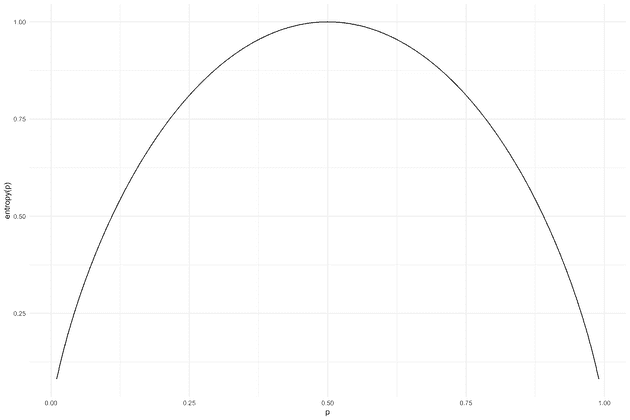
In general if there is an agreed upon scheme to determine which test to perform next, this defines an encoding of the string of $P_1P_2\ldots P_N$ and it can be uniquely decoded by simply inverting the process. Now we can use Shannon’s source coding theorem, that establishes the limits to possible data compression, e.g. how few tests do we need to determine the Covid-19 statuses. This comes down to the term “information”, a series of bits contain much information if it is highly unpredictable and conversely it has less information if it has a lot of redundancy. For this, we are gonna assume that all the tests are independent. This assumption would be violated if the tested individuals are family members or co-workers, in which case they are likely (positively) correlated. Under the assumption of independence the series of bits (tests) is maximally unpredictable, and hence has the highest information content, if there is a 50/50 chance of being 1 or 0 (positive or negative). The formula for computing information (for a single symbol) is

entropy <- function(p) {-p*log2(p)-(1-p)*log2(1-p)}
p <- seq(0.01, 0.99, 0.01)
qplot(x = p, y = entropy(p), geom = "line") + theme_minimal()

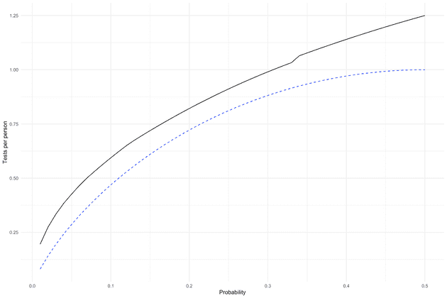
When $p=0.5$, $H(p)=1$, meaning that there is a lower bound on 1 bit (test) per individual. In other words, in that case there is no better strategy than just testing everyone individually. What allows the pooling strategy to work is that the positive percentage is much lower (in Denmark it has varied between 0.5%-4%), taking 1% as an example, the theoretical lower bound is only $H(0.01)=0.081$ tests per person.

This is a theoretical lower bound, in the scenario considered by Shannon any sequence of 0s and 1s could be used to compress an original sequence. Here we are bound by “1” meaning that some subset of test contain at least one “1”. It is clear to see that if the positive percentage was very high, the scheme would be useless even though information is symmetric - a series with 1% positives and a series with 99% positives have the same information content, but only the first can be “compressed” using this scheme.

How close can we get to the lower bound? Let us first try a simple method, first test a batch of $n$ persons, if they come out positive, we test each person in the batch individually. We choose the batch size $n$, so that it minimizes the expected number of tests per person given the positive probability $p$.

ps <- seq(0.01, 0.5, 0.01)

tests_per_person_method1 <- sapply(ps, function(p){
  ns <- seq(2, floor(1 / p))
  p_all_negative <- (1-p)^ns
  exp_tests <- p_all_negative * 1 + (1-p_all_negative) * (1+ns)
  
  tests_per_person <- exp_tests / ns
  
  min(tests_per_person)
})

How close does that get us to the lower bound? Below we see first strategy compared to the theoretical minimum (dashed blue line). While the absolute difference is not that large, the relative difference is large particularly for small $p$.

What should we do to get closer? Generally, we should aim to have each test provide as much information as possible. If $P_i$ again denotes the random status of individual $i$, and $T$ is a test of some of the individuals we can use conditional entropy to see that

The term $H(T|P_1\ldots P_N)$ is zero since the test status is known if we known the sequence of individual statuses. So we get

After having performed enough test that we know the sequence $P_1\ldots P_N$ the entropy is reduced to zero, so we should try to maximize $H(T)$. From before we know that $H(T)$ is maximized if $P(T) = 0.5$. With this philosophy, our second attempt is a bisection method. First, we choose the an initial batch size, so that the probability the test is positive (at least one positive in the batch) is a close to 50% as possible. If the test is negative we move on, otherwise we “bisect” the batch, i.e. test one half at a time, until we have identified a positive individual. Below I have simulated the expected number of tests per person. We can now compare the two methods:

run_test <- function(pool, first_cut) {
  determined <- rep(FALSE, length(pool))
  tests_used <- 0
  while(!all(determined)) {
    undetermined <- sum(!determined)
    to_test <- which(!determined)[1:min(undetermined, first_cut)]
    
    # Test pool
    if (any(pool[to_test] == 1)) {
      test <- at_least_one_positive(pool[to_test])
      determined[to_test] <- test$determined
      tests_used <- 1 + tests_used + test$tests_used
    }
    else {
      determined[to_test] <- TRUE
      tests_used <- 1 + tests_used      
    }
  }
  return(tests_used)
}

at_least_one_positive <- function(pool) {
  # Return determined, and number of tests used
  n <- length(pool)
  if (n == 1) {
    return(list(determined = TRUE,
                tests_used = 1))
  }
  if (n <= 3) {
    return(list(determined = rep(T, n),
                tests_used = ifelse(all(pool[1:(n-1)] == 0), n-1, n))) # if all the first are negative the last is positive without testing
  }

  cut <- floor(n/2)
  
  # Test 1st half
  if (any(pool[1:cut] == 1)) { # has at least one positive
    test1 <- at_least_one_positive(pool[1:cut])    
    return(list(determined = c(test1$determined, rep(F, n - cut)),
                tests_used = test1$tests_used + 1))
  }
  # No-one positive in 1st half so test second
  else {
    test2 <- at_least_one_positive(pool[(cut+1):n])
    return(list(determined = c(rep(T,cut), test2$determined),
                tests_used = test2$tests_used + 1
           ))
  }
}

ps <- seq(0.01, 0.5, 0.01)
ns <- 100 / ps
tests_used_method2 <- sapply(ps, function(p) {
  N <- 100 / p
  replicate(400, {
    status <- rbinom(N, 1, p)
    first_cut <- ceiling(log(0.5)/log(1-p))
    run_test(status, first_cut)
  }) %>% mean
})

tests_per_person_method2 <- tests_used_method2 / ns

The above is obviously a (fun!) theoretical exercise, in practice there are many problems that hinder its use: Do the tests work if pooling too many people? Can the swab from one person be tested multiple times? Can we accept waiting for multiple tests before receiving an answer? The answer is probably “no”. Nonetheless, it is fun to see that Shannon’s theoretical framework of information can be applied in this unfamiliar setting of Covid-19 testing.