5 minutes - left who is winning?

In beach volleyball there is a serving disadvantage, the team receiving serve has a higher than 50% probability of winning while receiving (also called “siding out”). This makes for exciting end-games with a lot of back and forth. If the game is tied at 14-14 in the deciding set, we can use Markov chain theory to workout the probabilities that either team will win. The other day I watched a match on YouTube and found to my surprise that there were still 8 mins left on the video at the score 14-14. What happens to the winning probabilities if we have this additional information on the time left on the clock?
Let’s start by considering the problem where we ignore the information about how much time is left and only consider the score. In that case we have a Markov chain with 6 states; winning, leading by one serving, tied receiving, tied serving, trailing by one receiving and loosing.
Let the probability of winning while receiving (“siding-out”) be p and the probability of winning while serving be q = 1 − p, then the transition matrix, Q, for the Markov chain is:
Note that the two states “Winning” and “Loosing” are so-called “absorbing” states if you have lost you can not un-loose - you have been absorbed in the loosing state and will remain there eternally.
p1 <- 0.7 # side-out probability team1
q1 <- 1-p1
p2 <- 0.7 # side-out probability team2
q2 <- 1-p2
transition <- matrix(c(1, 0, 0, 0, 0, 0,    # WINNING
                       q2, 0, p2, 0, 0, 0,  # +1 (SERVING)
                       0, p1, 0, 0, q1, 0,  # 0 RECEIVING
                       0, q2, 0, 0, p2, 0,  # 0 SERVING
                       0, 0, 0, p1, 0, q1,  # -1 (RECEIVING)
                       0, 0, 0, 0, 0, 1),   # LOOSING
                     nrow = 6, ncol = 6, byrow = TRUE)
Now still without considering the time left on the video, we can compute the probability of eventually winning given the current state, by finding the limit limn → ∞Qn. This can be done algebraically, but practically it is easier to just compute Qn for a sufficiently large n.
(transition %^% 10000)

##           [,1] [,2] [,3] [,4] [,5]      [,6]
## [1,] 1.0000000    0    0    0    0 0.0000000
## [2,] 0.7083333    0    0    0    0 0.2916667
## [3,] 0.5833333    0    0    0    0 0.4166667
## [4,] 0.4166667    0    0    0    0 0.5833333
## [5,] 0.2916667    0    0    0    0 0.7083333
## [6,] 0.0000000    0    0    0    0 1.0000000
The probability of winning for each initial state, can be read in the first column of the matrix above, for instance the chance of winning is 70.8% if leading by one and serving and 58% if tied and receiving.
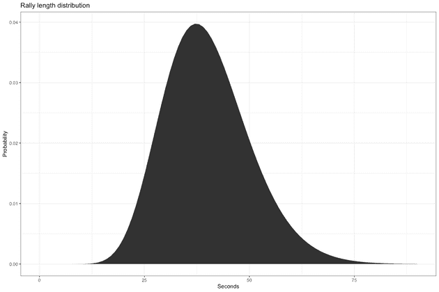
Now we complicate the problem by adding information about the average rally length - infact - it is not the average rally length but rather the total time between consecutive serves. We will model it using a gamma distribution, with parameters and . This gives a mean rally length of 40 seconds:
rally_length_alpha <- 15
rally_length_beta <- rally_length_alpha / 40

qplot(x = seq(0, 90, 1),
      y = dgamma(seq(0, 90, 1), shape = rally_length_alpha, rate = rally_length_beta),
      geom = "area") +
  theme_bw() +
  ggtitle("Rally length distribution") +
  xlab("Seconds") +
  ylab("Probability")
To compute
Furthermore,
The variable T = t ∣ R = r is simply a sum of independent gamma distributed variables, which itself is gamma distributed with parameters αr = r**α and β = β. The quantity P(R=r) can be found as the probability that the Markov chain is fixed after steps, minus the probability that it has been fixed in less than steps:
Where is the initial state. is a normalizing constant and is most easily computed by simply summing . The probability of winning after exactly r rallies, can be computed as
And by Bayes’ formula:
We now have everything we need to compute P(W | T = t):
time_left_seq <- seq(0, 60 * 10, 5)
win_prob <- function(transition, time_left_seq) {
  init_state <- c(0, 0, 1, 0, 0, 0) # 0 RECEIVING
  win_prob_seq <- c()
  for (time_left in time_left_seq) {
    rallys_left_seq <- seq(2, 40, 2)

    rallys_left_prob <- dgamma(time_left, shape = rallys_left_seq * rally_length_alpha, rate = rally_length_beta)

    for (rallys_left_idx in seq_along(rallys_left_seq)) {
      rallys_left <- rallys_left_seq[rallys_left_idx]
      prob_game_over_prev <- sum((init_state %*% (transition %^% (rallys_left-2)))[1, c(1,6)]) # Probability game-over before
      prob_game_over_now <- sum((init_state %*% (transition %^% (rallys_left)))[1, c(1,6)]) # Probability game-over now
      rallys_left_prob[rallys_left_idx] <- (prob_game_over_now - prob_game_over_prev) * rallys_left_prob[rallys_left_idx]
    }

    # P(R = r | T = t)
    rallys_left_prob <- rallys_left_prob / sum(rallys_left_prob)

    win_prob <- 0
    for (rallys_left_idx in seq_along(rallys_left_seq)) {
      rallys_left <- rallys_left_seq[rallys_left_idx]
      prob_win_lose <- -((init_state %*% (transition %^% (rallys_left-2)))[1, c(1,6)]) + (init_state %*% (transition %^% (rallys_left)))[1, c(1,6)]

      # P(W | R = r)
      prob_win_lose <- prob_win_lose / sum(prob_win_lose)

      win_prob <- win_prob + prob_win_lose[1] * rallys_left_prob[rallys_left_idx]
    }

    win_prob_seq <- c(win_prob_seq, win_prob)
  }
  return(win_prob_seq)
}

win_prob_seq <- win_prob(transition, time_left_seq)

qplot(x = time_left_seq, y = win_prob_seq, geom = "line") + theme_bw() +
  xlab("Time left in seconds") +
  ylab("Probability of winning")
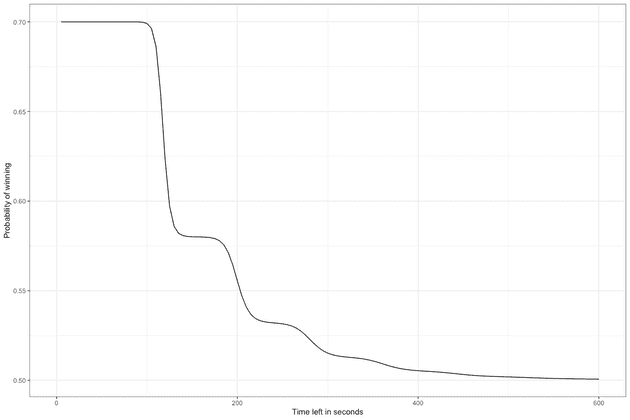
Note the “bumps” in the winning probability, corresponding to times where there is a switch between the most likely number of ralleys left. We can also see that the 58% percent advantage there was to being tied 14-14 receiving, has been reduced to practically nothing (50%) with 8 minutes left on the clock.
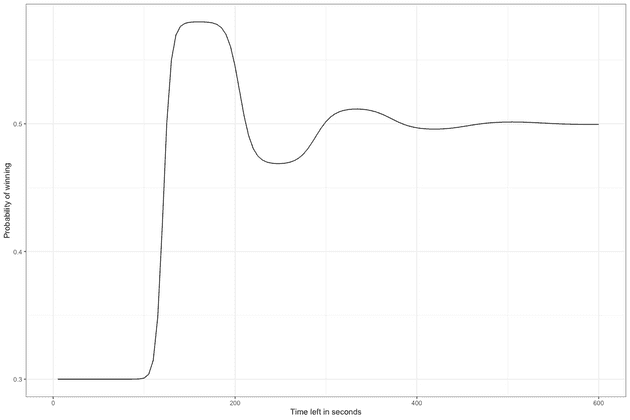
If it had been the other way around, that servers had an advantage the curve gets even more interesting, oscilating between favouring the first team, then the second, etc.
p1 <- 0.3 # side-out probability team1
q1 <- 1-p1
p2 <- 0.3 # side-out probability team2
q2 <- 1-p2
transition <- matrix(c(1, 0, 0, 0, 0, 0,    # WINNING
                       q2, 0, p2, 0, 0, 0,  # +1 (SERVING)
                       0, p1, 0, 0, q1, 0,  # 0 RECEIVING
                       0, q2, 0, 0, p2, 0,  # 0 SERVING
                       0, 0, 0, p1, 0, q1,  # -1 (RECEIVING)
                       0, 0, 0, 0, 0, 1),   # LOOSING
                     nrow = 6, ncol = 6, byrow = TRUE)
win_prob_seq <- win_prob(transition, time_left_seq)

qplot(x = time_left_seq, y = win_prob_seq, geom = "line") + theme_bw() +
  xlab("Time left in seconds") +
  ylab("Probability of winning")

